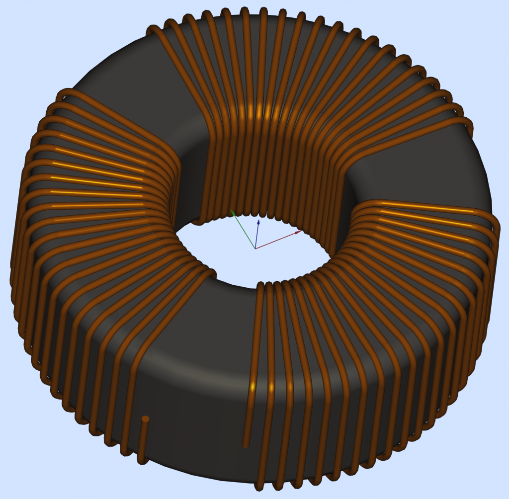
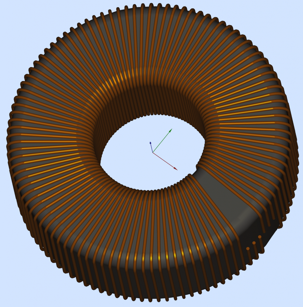
Finally, I completed my first 3D Toroidal Winding Project in FreeCAD, and I can use it for real work. Just changing a few numbers in a spreadsheet I can generate automatically and in only a few seconds pretty much any transformer configuration, up to 32 layers/windings, based on real spec-sheet core and winding wire parameters. With a bit of COPY/PASTE it is possible to add more winding layers, more windings in a layer, change independently the beginning/end angle of the windings, the winding pass, interleave or separate them, and so on.

What was so difficult you ask?

For starters, I had to learn a CAD program. And yes, FreeCAD has some impressive abilities; dealing with a bunch of Toroidal windings is not one of them, or at least it was not quite trivial starting with a Helix. There is a good tutorial on YouTube, and it helped me to understand the good and the not so good: https://www.youtube.com/watch?v=ou92FEz1lT0 . Without too much talking, the working projects can be found here:

How I did it?

The secret sauce I used to get a “perfect” 3D model was to avoid altogether the Helix beast and to describe the winding contour on the toroid based on only straight lines and perfect circles. Feeding FreeCAD with only this kind of elementary data proved to be the right medicine. Many thanks to chrisb and to drmacro from the FreeCAD forum, they clarified where I should look for problems. Now the size of the project file, the precision of the model, and the FreeCAD processing speed are quite ideal I would say.

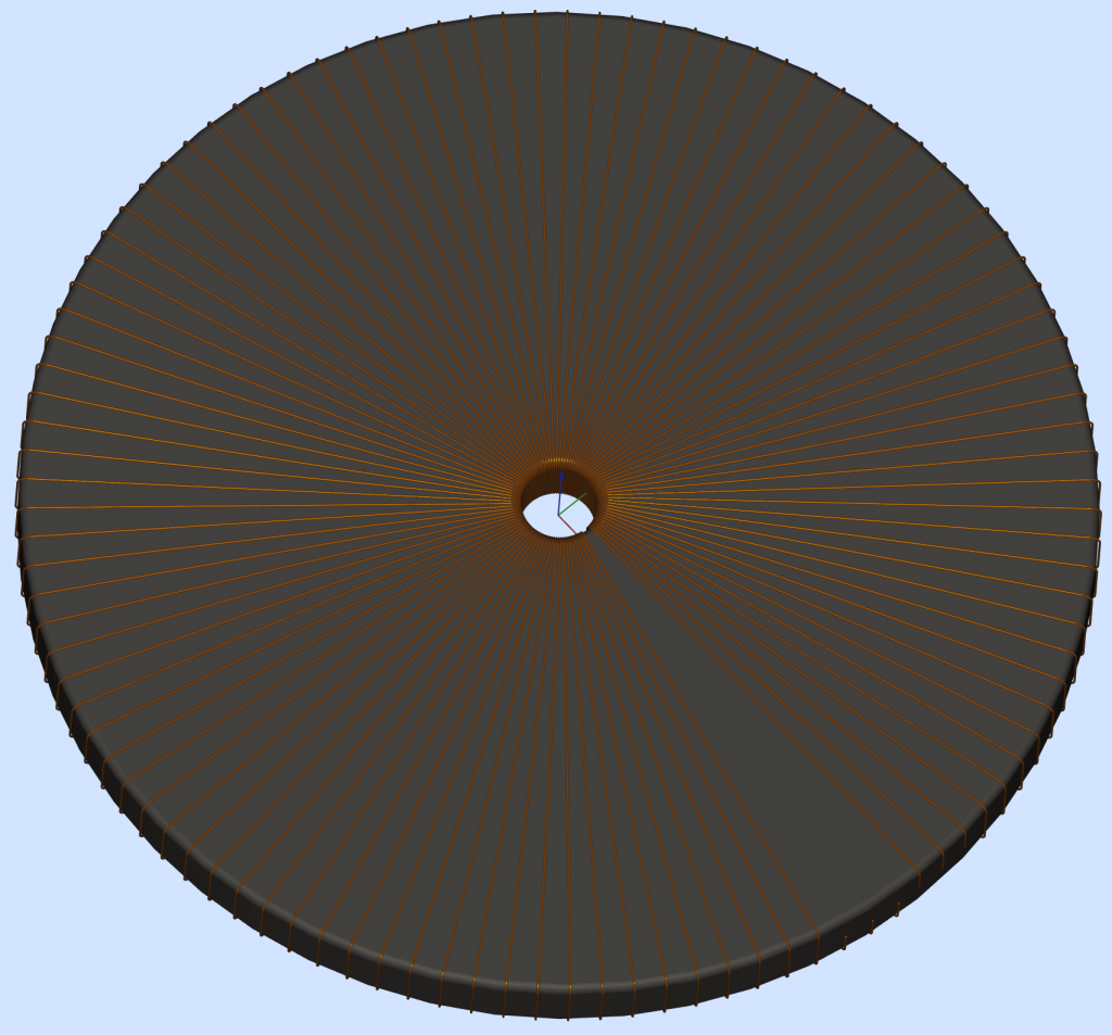
The winding head has guiding pads to keep the wire in a defined position, especially when the sliding belt or the shuttle are in the “recovery” arc. This winding technique will force the wire to follow a mostly vertical path on the outside or the inside surface, while the angle progression from turn to turn is mostly placed on the TOP and the BOTTOM surface of the Torus. The 3D model proposed here is using vertical planes arranged to mark the winding reference angles. The winding path traced on the vertical Torus surfaces will have vertical lines, and properly adjusted winding angles on the flat TOP and BOTTOM surfaces. The proper dimensions and angles will be retrieved from the SETdata spreadsheet.

It is true, the “real” winding has some angle added on the internal and external vertical faces too. For the reason explained before this angle dos not quite follows an ideal Helix, and my model can be amended to account even for this slight mismatch (using 4 slicing planes instead of only 2). A winding machine will always wiggle over those angles, I decided that my 3D model falls inside the nominal winding precision window.

After the real Torus was defined I needed to define a new and larger Torus to help draw the path of the winding wire, more precisely the path for the center of the wire cross section. If more than one winding layer is required it is possible to define more and incrementally larger Torus shapes, to account for filling-up the Torus with multiple layers.

What was wrong with the YouTube tutorial?

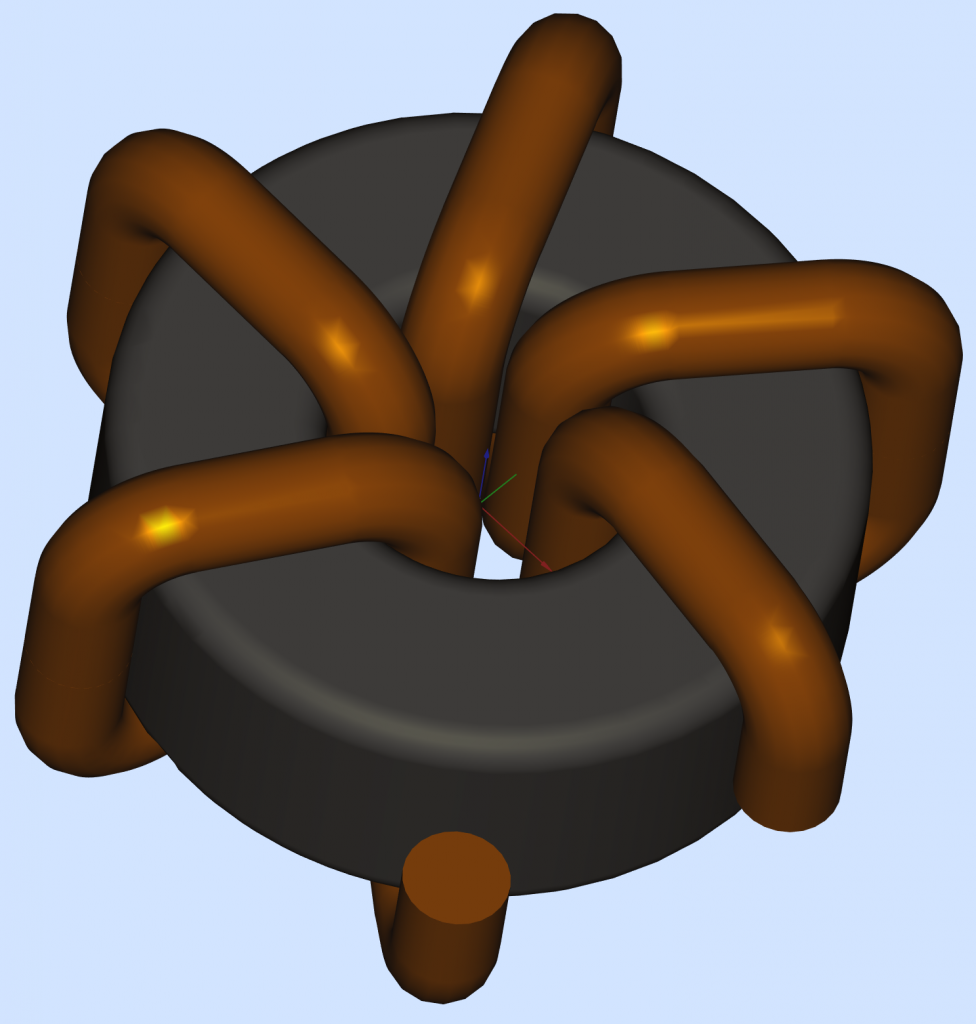
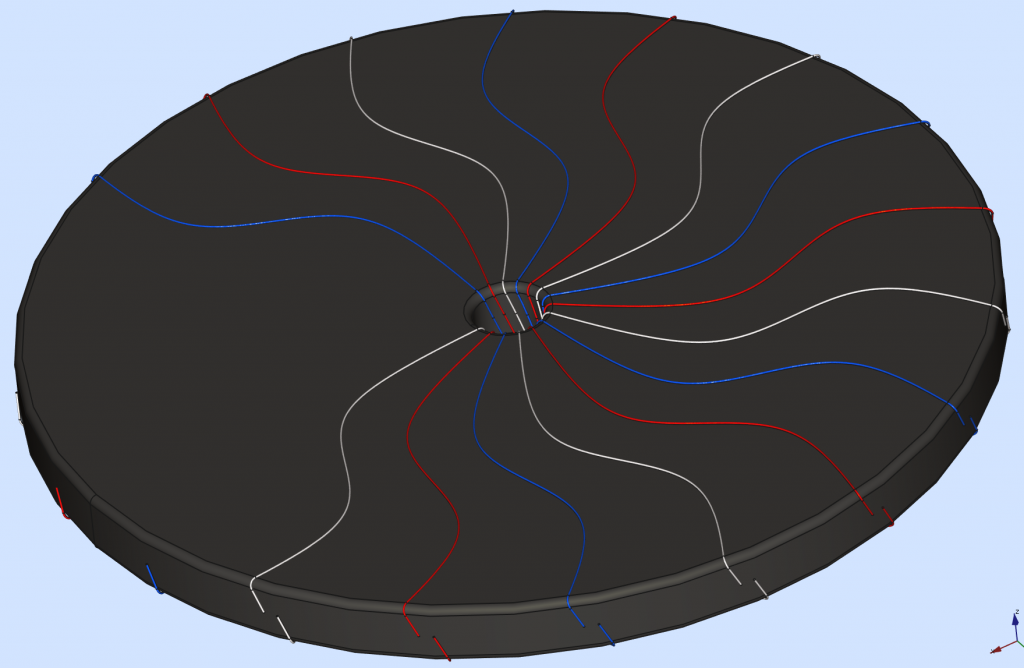
FreeCAD can easily create a Helix, but only if the Helix is progressing in a linear direction. Unfortunately, in order to place a Helical winding on a Torus you have to bend the Helix progression in a revolving way along the Torus. That, right there, is breaking the FreeCAD camel’s back: bending the Helix will dramatically increase the size of the FreeCAD project file, and the resulting shapes are kind of useless. Any attempt to further process those resulting shapes will crash the program after a looooong waiting time. And yes, poor FreeCAD will successfully check the geometry and it will report that everything is just peachy. The “work-around” used in the YouTube tutorial was to approximate a circular revolving Helix slice using a linear progressing Helix chunk. This choice works somehow, but only for “golden ratio” projects. As soon as one attempts to decrease the number of turns or to choose an unusual core size ratio, the 3D model kind of breaks down:

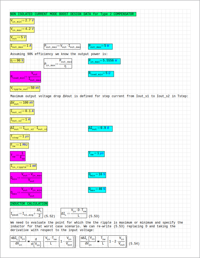
Current Mode BOOST Converter

Howdy, welcome to my den! This is the place for various projects to be shared with like minded people.
Open source? Use this stuff if you take full responsibility, and give to Daddyzaur what’s Daddyzaur’s.

So, are you an electrical engineer working with SPICE tools, designing real power supplies? Or you’re a hobbyist and you really want to build a Current Mode BOOST converter, but nobody put together some step-by-step instructions you can use for your project? If so, keep reading.

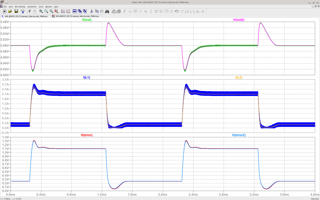
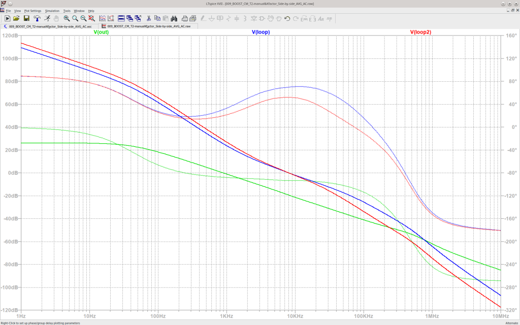
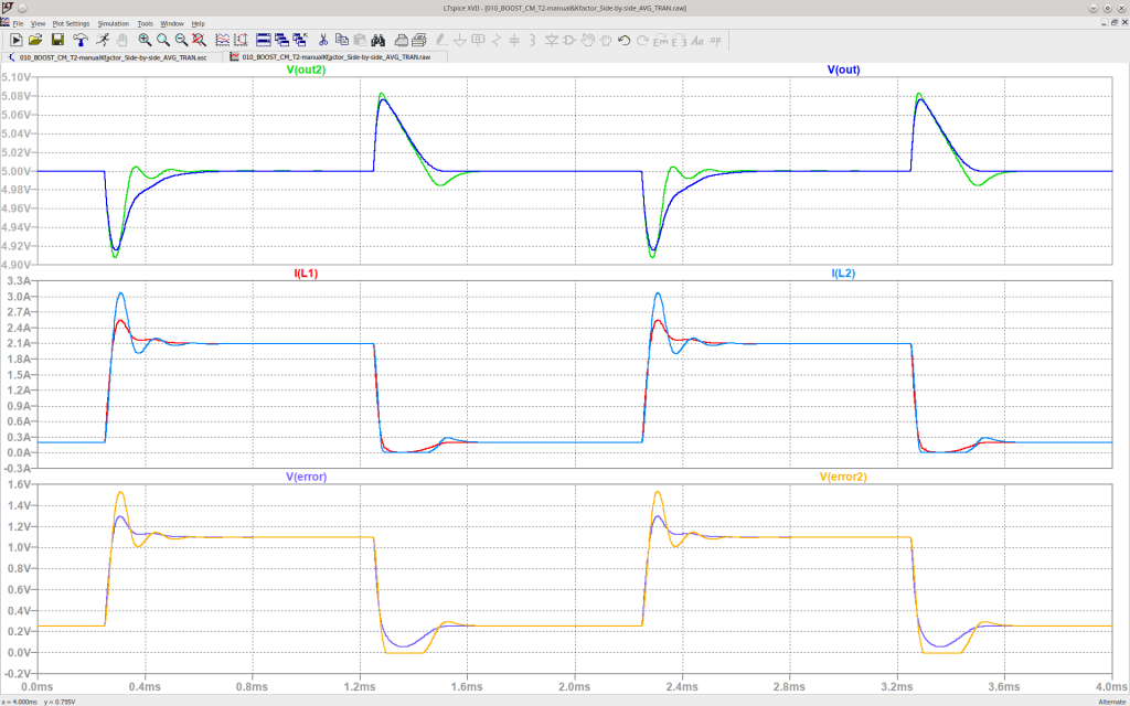
You will find here some explanations and an archive with all you need to get you started. You will get a high degree of confidence on your design, after seeing a perfect match between the average and switch mode models, compared throughout various Transient and AC simulations, under various conditions, with side-by-side perfectly matching signals.

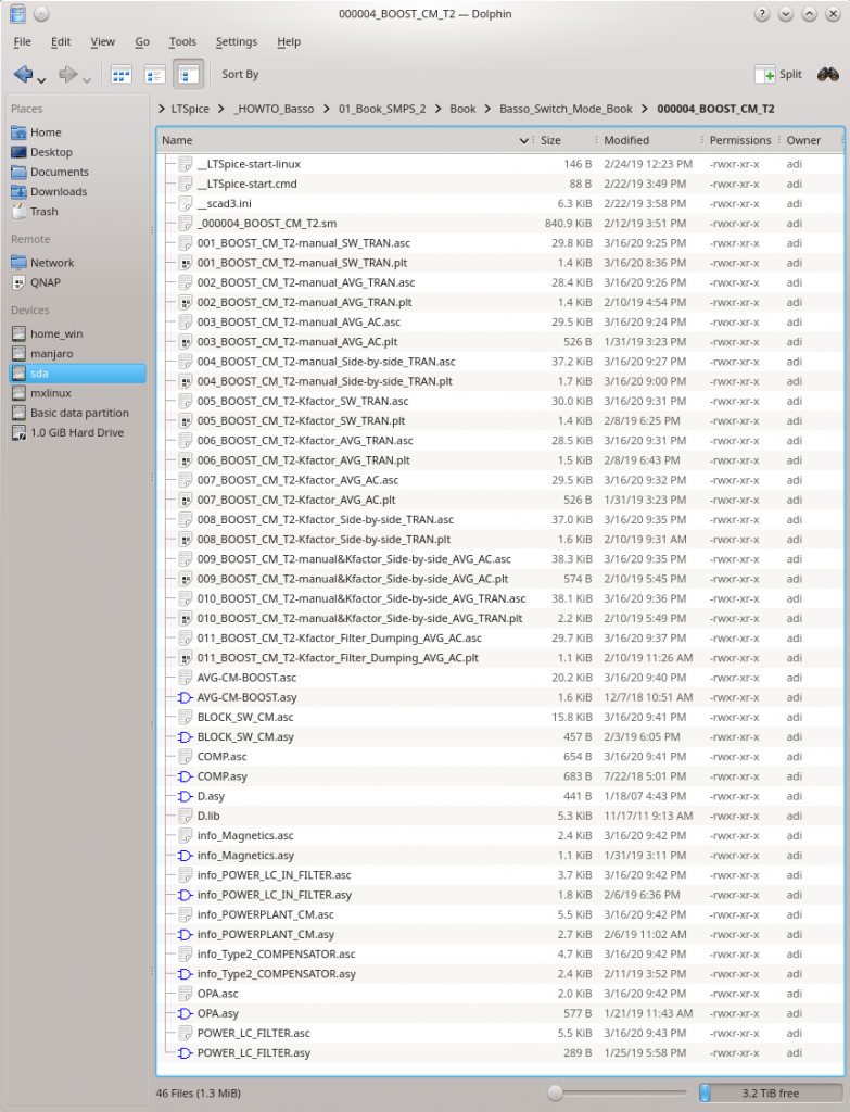
In the archive I provided are all the symbols, models and sub-circuits, included in one single project folder. You also need to install Smath Studio and LTSpice. You do not need to litter external folders with bits and pieces of your project files: the project folder is Self Contained, you can place it anywhere you like and it will just work, in Linux or Windows:

Part 4 of my Do you Power SPICE mini series is an example of a Current Mode Control BOOST Converter one can analyze and build with confidence, using an interactive set of SPICE and math tools. Usually, this type of application will employ a Type 2 Compensator. I put together those tools using mostly the excellent books written by Christophe Basso, and I tried to follow his work as close as possible. If you do not know who I am talking about go ahead and check his books:

https://www.amazon.com/Christophe-P.-Basso/e/B001IOH604%3F

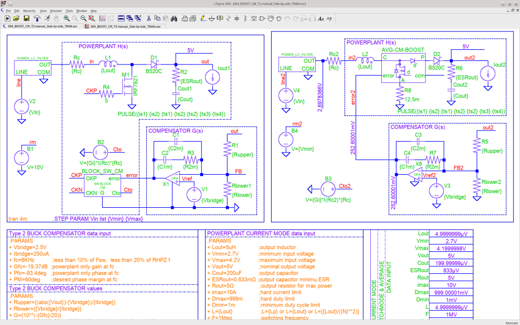
The starting point must always be a complete list with requirements for you converter: most everybody would agree, it is a good idea to know beforehand what you need. For this part you will find in my archive a Smath Studio design file _000004_BOOST_CM_T2.sm you can use to plug-in your data input and compute the parameters for SPICE. I tried to keep a resemblance of some rules: GREEN fields are title, YELLOW fields are usually for data input, RED fields are resulting parameters, BLUE fields are resulting quantities, and colorless fields are computing fields.

Now that you’ve got the input data and the SPICE parameters, go ahead and modify the LTSpice project files, with your data. The secret sauce for this flexibility is an (almost) identical interface I placed in every schematic with PARAMS for every and all variables you will need, and visual blocks for computed values. I said ALMOST because some of the .IC statements should be sometimes disabled or adjusted as required for the side-by-side sub-projects. Otherwise, nothing should be different. You can copy and paste this PARAMS block in all those LTSpice sub-projects, just verify the .IC statements:

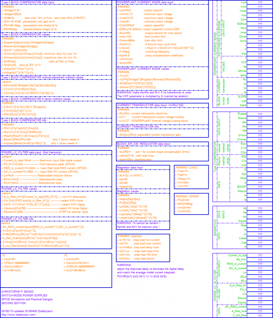
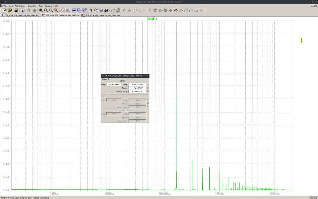
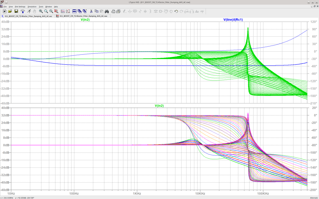
Go ahead, open the project files one by one and study them. You will find here almost everything for the transient and the AC analysis you need to design a stable control loop. Here is a summary with the SPICE sub-projects name convention: CM stands for Current Mode, T2 for Type 2 Compensator, SW for Switch Mode Models, AVG for Average Models, TRAN for Transient Simulation, manual for the manual method of placing poles and zeroes, Kfactor for the automatic K factor method, AC for the AC Simulation, and finally Side-by-side indicates the project file contains two circuits you can compare together, in a single simulation: